Realtime metrics with AWS IoT Analytics and CloudWatch

IoT Analytics is great for doing analysis of your IOT device data on a regular cadence, for example daily or hourly. Faster scheduled analysis is possible, and the minimum scheduling frequency was lowered to 15 minutes in August this year, but what if you want something near real-time? Although there isn’t a built in feature for this, if you just want to setup a basic alarm or build some straightforward near real-time dashboards, there’s a simple solution using the power of the IoT Analytics Lambda Activity coupled with AWS CloudWatch.

Messages from my devices flow into AWS IoT Analytics from a number of MQTT topics that are all routed to a Channel using Rules that I’ve setup with AWS IoT.

Data flowing into a Channel passes through a Pipeline before reaching the Datastore and this Pipeline is the key to getting our near real-time metrics.

The Lambda Activity in AWS IoT Analytics

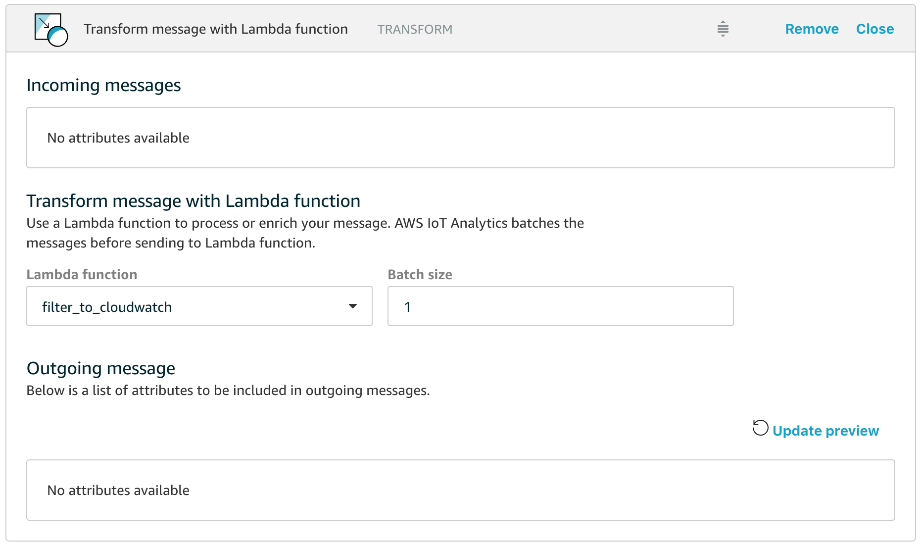
All we have to do is add a Lambda function into our Pipeline and have the Lambda function route appropriate data to AWS CloudWatch so that we can then use all the features of CloudWatch for building our dashboards, configuring alarms and combining our new custom metrics with data from other sources. In the example above, I’ve named the Lambda function filter_to_cloudwatch and let’s take a closer look at how simple this function can be.

import json
import boto3

def cw(topic,value,name):
 cloudwatch = boto3.client('cloudwatch')
 cloudwatch.put_metric_data( MetricData=[ 
 {
  'MetricName': name,
  'Dimensions': [{'Name': 'topic','Value': topic}],
  'Unit': 'None', 
  'Value': value
 }],Namespace='Telescope/Monitoring-Test')
 return

def lambda_handler(event, context):
 for e in event:
  if 'uptime' in e :
   cw(e["full_topic"],e["uptime"],"uptime")
  if 'illumination' in e :
   cw(e["full_topic"],e["illumination"],"illumination")
  if 'temperature' in e :
   cw(e["full_topic"],e["temperature"],"temperature")
 return event

Yes, that is all of the code, it really is that short.

Hopefully the code is self-explanatory, but in essence what happens is that the Lambda function in a Pipeline is passed an array of messages with the size of the array dependent on the batch size that you configure for the activity (the default of 1 means that the Lambda function will be invoked for each individual message, which is fine for scenarios where messages only arrive in the channel every few seconds).

The handler then loops through all the messages and looks to see if the message has attributes for uptime, illumination or temperature – these are the attributes that I want to graph in near real-time in this example. If the attribute exists in the message, we call the cw() function to emit the custom metric to AWS CloudWatch.

Note that the Lambda function simply returns the messages that it received so that they flow through the rest of the Pipeline.

Probably the biggest gotcha is that you need to make sure you have granted IoT Analytics permission to invoke your Lambda function, and you can do this with the following simple AWS CLI command.

aws lambda add-permission --function-name filter_to_cloudwatch --statement-id filter_to_cloudwatch_perms --principal iotanalytics.amazonaws.com --action lambda:InvokeFunction

If you forget this, and you have configured your logging options, you’ll see error messages like this for your cloudwatch log stream aws/iotanalytics/pipelines

[ERROR] Unable to execute Lambda function due to insufficient permissions; dropping the messages, number of messages dropped : 1, functionArn : arn:aws:lambda:us-west-2:<accountid>:function:filter_to_cloudwatch

And that’s it! We can now use all the loveliness of AWS CloudWatch to plot our custom metrics on graphs and dashboards with fine grained time resolution, for example this is a graph of my data every 30 seconds.

Example real-time metrics from the IoT Analytics Pipeline showing in CloudWatch

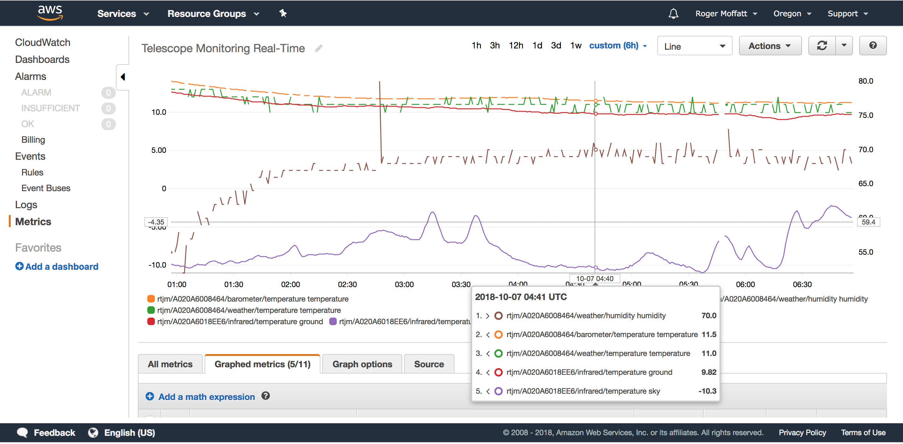
In conclusion, we’ve seen that with a little lateral thinking, we can leverage the Lambda Activity that is available in the AWS IoT Analytics Pipeline to route just the message attributes we want to a near real-time dashboard in AWS CloudWatch.

Happy Dashboarding!

Data Exploration with Amazon Quicksight and IoT Analytics

We discussed previously how to get data out of your data store by writing SQL queries to produce data sets in CSV format. What about exploring and visualising that data to make insights easier? In this post I’ll talk about the native integration between AWS IoT Analytics and Amazon QuickSight that makes this possible and fun.

First, let’s take a quick look at one of my dashboards.

This shows a variety of data about some of the sensors located in our garden (the locations on the map are not real) and as you can see it does a decent job of visualising the data at hand – but where does that data actually come from?

QuickSight has native support for AWS IoT Analytics Datasets and so your starting point is to create a new QuickSight Dataset using the Data Source selection page that looks like this.

Once you’ve selected a data set in IoT Analytics (remember, a data set is the result of a SQL query against the data store) you have some pretty nice data preparation tools in QuickSight that let you alter column types and even create new calculated columns – and this is an especially useful feature as you can, for example, take a unix timestamp and convert it into a date time object that QuickSight can use as the x-axis on many of your graphs. I wrote more about this here.

Quick Tip – turning strings into Geo-Coordinates for Amazon QuickSight

Some of my IoT projects report location data with messages that looks like this;

{
  "time": "20181007T071731Z",
  "kph": 0.01852,
  "alt": 140.1,
  "satellites": 11,
  "hdop": 75,
  "pos": [
    "47.64",
    "-122.36"
  ],
  "age": 379,
  "chk_f": 9,
  "chk_s": 46175,
  "fix": 10735
}

Notice how the co-ordinates are returned as an array of two strings where each string contains a decimal degrees value.

It’s clear what the data means, but for Amazon QuickSight to plot it on a map, it needs to have this coordinate expressed in the correct type – in this case a Geo coordinate.

As I mentioned before, we can use a QuickSight calculated field to solve this problem. This time the formula we need is a little more complex but in essence we are going to split the string into 2 and use one part for a Latitude Geo Coordinate and the other for a Longitude Geo Coordinate.

Here’s the calculated field formula for the Latitude

parseDecimal(split(replace(replace({pos},"[",""),"]",""),",",1))

And here’s the almost identical one for the Longitude (which uses the second array value rather than the first)

parseDecimal(split(replace(replace({pos},"[",""),"]",""),",",2))

These calculated fields will be numbers to start with, we still need to tell QuickSight that we want to treat these as coordinates suitable for mapping, so  use the edit data type feature to convert them to the appropriate Geo type like this.

Once you have Latitude and Longitude fields, you’ll be able to visualise them on the map charts built in to QuickSight.

A natural home for your IOT Data – AWS IoT Analytics

IoT devices send a wide range of message shapes and sizes, and for my own experiments, I typically send a different type of message for each sensor. So for example;

Cloud Sensor Message

{
  "ambient": 9.649988,
  "object": -2.509985,
  "unit": "Celcius",
  "epoch": 1538896592,
  "status": {
    "uptime": 88,
    "heap": 15488,
    "unit": "minute",
    "rssi": -71
  }
}

Temperature Sensor Message

{
  "temperature": 10,
  "unit": "Celcius",
  "epoch": 1538896611
}

GPS Location  Message

{
  "time": "20181007T071731Z",
  "kph": 0.01852,
  "alt": 140.1,
  "satellites": 11,
  "hdop": 75,
  "pos": [
    "47.64",
    "-122.36"
  ],
  "age": 379,
  "chk_f": 9,
  "chk_s": 46175,
  "fix": 10735
}

I have maybe 20-30 different messages in my small home automation setup and I’d like the freedom to be able to create new message formats without having to worry about how to store all this data for later analysis, so one of the first questions that arises is where should I store all this data?

A natural destination for any IOT device data is the new IoT Analytics service that was launched by AWS back in April at the world’s largest industrial technology trade fair “Hannover Messe”. IoT Analytics has several features that make the collection and later analysis of connected device data easy;

Flexible retention periods. Keep all your data for a week, a month or any period that you require, including of course unlimited retention. Aside from helping reduce costs by automatically removing old and non longer needed data, this also helps keep query performance higher by lowering the overall amount of data being scanned.

Zero schema configuration required. You don’t need to specify any partition keys or column names or tell IoT Analytics anything about your message schema. Just send the data and it will be stored and made available for query. I like this because it makes it super easy to get up and running.

Preprocess message data before storage. IoT Analytics has a Pipeline that connects the incoming messages from a Channel to the Datastore – your data lake of connected device data. This gives me a data preparation step where I can enrich or transform the message according to my requirements. For example I might want to enrich the message with data from the IoT device shadow or add information from the IoT device registry. I might want to convert a measurement in fahrenheit to celcius or even call out to an external service to get some additional data about the device to add to the message. There are some pretty cool things you can do with the data preparation stage and I’ll write more about those another time.

Ability to write standard SQL queries against your data. I call this out in particular because prior to the release of AWS IoT Analytics, I was using AWS ElasticSearch as my data repository. This had similar ease of use characteristics regarding schema configuration (not quite zero touch, but not particularly onerous either) and was certainly useful for visual analysis and deep diving with Kibana, but ES has it’s own query language based on Lucene and this makes decades of familiarity with SQL obsolete and having to learn how to query from the beginning was a learning curve that I sometimes found frustrating.

Recurring scheduled queries. One of my use cases concerns looking at historic and future weather data to determine when to turn on an irrigation system and for how long. I want to execute this analysis every evening to configure the watering for the next day – a perfect fit for a scheduled query that runs every day. Another use case I have is that of analysing upper atmosphere clarity to see if my telescope should continue to execute its observing program – a great fit for analysis that is scheduled to run every 15 minutes.

I love being able to automate my analysis like this without having to write a single line of code. This definitely makes my life easier when I’m wearing my data scientist hat.

And, saving the best for last …

Automated execution of Jupyter Notebooks for fully hands-off analysis workloads. For me, this is the real engine within IoT Analytics that makes it so flexible and capable. Not only can I use the notebook to perform deeper statistical analysis or train an ML scenario, or draw complex graphs and charts, but because I have the full power of the AWS SDK at my fingertips, I can do anything you can think of doing with all the tools that puts at your disposal. One simple use case I solve with this approach is to configure AWS CloudWatch Event Rules to schedule when water should be turned on and off and I’ll write more about this in some detail another time.

Example Jupyter Notebook fragment

In conclusion, the ease of sending any data in, the ability to query the data on an automated schedule and the power of the analysis available has enabled me to focus more on the business problems I’m trying to solve. For every new project I’m dreaming up (I’m an inveterate tinkerer remember), I just create a new IoT Analytics Channel->Pipeline->Datastore and that becomes the home for all the device data I’m sending.


Quick Tip – using unix timestamps or epochs in QuickSight

It’s not uncommon for IoT Devices to send timestamp information in simple integers like a unix timestamp or epoch. For example, the time of 10/08/2018 @ 1:05am (UTC) is represented by the epoch 1538960714 which is the number of seconds since Jan 1st 1970. Sometimes we might also have this in milliseconds, such as when we use an IoT Core Rule to add a timestamp to the incoming message.

If I have an AWS IoT Analytics Data Set containing epoch seconds or milliseconds, I’ll find it difficult to use that data effectively in Amazon QuickSight which really needs to have a date type column in order to consider it as a time. What to do?

This is where QuickSight’s ability to have calculated fields comes to the rescue.

Click on New field and then give your new field a name such as epochDate. Then you want to use the epochDate built in function to convert your epoch seconds or milliseconds data into the right format.

In this example my messages contain a field called received which is in epoch milliseconds, and so I’m dividing that by 1000, converting the result to an integer (required by the epochDate function) and then returning the result of the epochDate() function.

epochDate(decimalToInt({received}/1000))


Quick Tip – Dataset SQL – don’t forget __dt

When you create a Data Set with IoT Analytics, the default SQL query that is shown in the SQL editor is something like this;

SELECT * FROM datastore

Whilst there’s nothing wrong with this as a starting point, it’s important to realise that an unconstrained query like this will do a full table scan of your data every time it is executed. That may be OK if you have a short retention period configured for your datastore and you only have a few thousand messages, but imagine having terabytes of data stretching back over years and really you only want to get data for the last few days? The query above may work (it may also time out), but it’s vastly inefficient and you’ll be paying for the privilege of scanning the entire data store every time.

There is a better way.

Your first starting point should always be to use a WHERE clause referencing the system provided __dt column. For ‘dt’, think ‘datetime’ because it is this column that gives you access to the time based partitions that help you make queries on IoT Analytics and the double underscores are used to avoid clashes with any attribute names in your own data.

Here’s an example that just looks at data from the past day.

select * from telescope_data where __dt >= current_date - interval '1' day

__dt has a granularity of 1 day so if you want to look at a narrower time-range, you would add a constraint on whatever timestamp column you had in your data, but always, always, always include the __dt constraint as part of your where clause to maximise query performance and lower query cost.

For example, what if we just want data from the last 15 minutes in our query results?

select * from telescope_data where __dt >= current_date - interval '1' day 
and from_unixtime(epoch) > now() - interval '15' minute

Notice that we have the __dt clause to restrict data to the most recent day and then have a clause based on the epoch reported in each message to further restrict to the last 15 minutes.

Adding a timestamp to messages from devices that have no clocks

Small remote sensors may not send a timestamp with every message and this can make later processing and analysis a challenge. Typically you want to think of IoT Data as being a time-series and there’s a bit of a clue in that name.

So how do we cope with messages that don’t have any hint of a timestamp?

This where the power of the IoT Core Rule comes to play. You will recall that so far we’ve seen rules that look like this;

SELECT * FROM 'rtjm/#'

This rule selects everything arriving on the rtjm/# topic space and sends it on to the destination. But what if we extended this to add in additional information? For example, we can add in the arrival time of the message like this;

SELECT *,timestamp() as received FROM 'rtjm/#'

We’re still using the * as before, but now we’re adding the current timestamp and naming it as a new attribute –  ‘received’ – in the message. Sorted!

That’s not all though. What about passing on the topic the messages are received on as well? This can be useful if your device id is contained in the topic rather than the payload of the message for example. How about this for example;

SELECT *,topic() as full_topic, timestamp() as received FROM 'rtjm/#'

This is just scratching the surface of course, for a full list of the capabilities, head on over to the AWS IoT Core documentation on SQL